Basic questions regarding option pricing with FDM

[Pehr]

When calculating the option prices with the use of finite difference methods you approximate the derivatives in the Black & Scholes PDE.
Where do you get the option prices used in these approximations? I mean, we are supposed to calculate the option price, and at the same time you need prices to do the approximations of the derivatives.
Also, what is x in the BS PDE du/dt = 1/2 * sigma^2 * d^u/dx^2?

Thanks in advance.

 

[Steven]

You need the boundary condition, i.e. the payoff function, to start off the calculation. Read the method carefully.
x is the underlying asset.

 

[Daniel Duffy]

You need the boundary condition, i.e. the payoff function, to start off the calculation. Read the method carefully.
x is the underlying asset.

This is the initial/payoff function and is not a BC, really.

You need 2 numerical boundary conditions to make the problem solvable:

. when S = 0 (near field)
. when S = Smax (far field)

You need to estimate Smax (domain truncation) and then BCs for call and put cases.

I posted an example elsewhere for your same question.

 

[Alexei]

This is the initial/payoff function and is not a BC, really.

You need 2 numerical boundary conditions to make the problem solvable:

. when S = 0 (near field)
. when S = Smax (far field)

You need to estimate Smax (domain truncation) and then BCs for call and put cases.

I posted an example elsewhere for your same question.

Domain truncation can be estimated based on statistical significance.

 

[Daniel Duffy]

This is the initial/payoff function and is not a BC, really.

You need 2 numerical boundary conditions to make the problem solvable:

. when S = 0 (near field)
. when S = Smax (far field)


Domain truncation can be estimated based on statistical significance.

The results of Kangro can be used to compute this. But there is a more accurate way and the resulting BCs are easy to find: we use domain transformation (e.g. y = S/(S+K)) and the Fichera boundary conditions. So, no truncation error, and when used with ADE method the result is very accurate. It's all documented.

 

[weiwern]

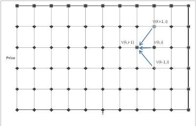
I think you posted this question on another forum as well. But if you look at this here, it pretty much describes what I'm trying to explain http://4.bp.blogspot.com/_3E_7nRJs1Mw/TDC7UNeZw9I/AAAAAAAAEMc/R2G2vKji3hs/s400/Untitled.jpg

I like to think of the FDM method (explicit one specifically) to be similar to the binomial model. I think this paper here shows it to be so
http://www.haas.berkeley.edu/groups/finance/WP/rpf292.pdf

 

[Daniel Duffy]

Yes, I posted.

Well, I think drawing analogies between lattice method and FDM will break down at some stage in my opinion. They have different properties.

The mathematical basis of FDM is well-developed, has been known and used for 200 years and has a huge literature. I would suggest learning without leaning on lattice methods, it becomes confusing at some stage. Or stick to lattice.

The binomial method is useful for motivating.

 

[Pehr]

I still don't understand where you get S from. You guys say that you start off at the end point (at time T) because you know the payoff VK(S, T) = max(S - K, 0) at this point in time. But how do you know all the different underlying asset prices S at the time point T (and all other time points)? In the explicit FDM you need Sj-1, Sj and Sj+1 (all at time i+1) to calculate the price at time i.

 

[weiwern]

I agree with your point Daniel.

Pehr, we determine the underlying asset price S at the end points by first assuming an upperbound for S ((S_{max}=2*Strike) or something along those lines) and a lowerbound (S_{min}=0). Then we divide (\delta S={(S_{max}-S_{min})}/{N}) to get our asset steps and so now we have asset values (S_i=i\delta S) for (0\le i \le N) along the grid.